2 Background and Research Question

Our analysis picks up on the suggestion of Ding and Li (Reference Ding and Li2019), who conclude with the open question of how the bracketing property would extend to a model that incorporates both FE and a LDV (we refer to this as the “FE-LDV model”).Footnote ³ Although the FE-LDV model simultaneously controls for time-invariant unobserved heterogeneity and the feedback effect, its estimation requires stronger assumptions than either the FE or LDV models individually, a point recognized by Ding and Li (Reference Ding and Li2019).

Indeed, the appeal of the bracketing property lies in its inherent promise to be an alternative to estimating the FE-LDV model, for which estimation will suffer from “Nickell bias” if the number of time periods is fixed (Nickell Reference Nickell1981).Footnote ⁴ Under these circumstances, a Generalized Method of Moments approach in the style of the Arellano and Bond (Reference Arellano and Bond1991) estimator (AB estimator) is a common way to obtain a consistent estimate of the treatment effect, $\tau $ .Footnote ⁵ However, as the AB estimator instruments the lagged dependent variable, $y_{i,t-1}$ , with deeper lags of $y_{it}$ , the method requires the availability of sufficient time periods. Additionally, the deeper lags of $y_{it}$ need to be strong instruments for $y_{i,t-1}$ , which may render the AB estimator inapplicable in many cases. Leszczensky and Wolbring (Reference Leszczensky and Wolbring2022) discuss several of the challenges in applying the AB estimator, including downward bias in the face of a large number of moment conditions (Hsiao Reference Hsiao2022), weak instruments problems (Bun and Windmeijer Reference Bun and Windmeijer2010), and poor finite-sample performance (Moral-Benito et al. Reference Moral-Benito, Allison and Williams2019).

The bracketing property afforded by separate estimation of FE and LDV models avoids these complexities, and covers the circumstance when unobserved heterogeneity or feedback effects of the lagged outcome on the treatment are deemed threats to identification. This cuts to the issue raised by Ding and Li (Reference Ding and Li2019): Their analysis, along with that of Guryan (Reference Guryan2001) and Angrist and Pischke (Reference Angrist and Pischke2009), applies to the situation in which either the assumption underlying the FE model or the assumption underlying the LDV model is fulfilled. But given a concern for the validity of each assumption individually, the question arises as to the consequences for bracketing when the assumptions are simultaneously violated.

3 Biases in Case of Feedback and Endogeneity

An insightful case in which the assumptions of the FE model and the LDV model are violated is given by a DGP in which both the outcome variable y and the explanatory variable of interest x are functions of individual time-invariant factors $\alpha _i$ , that is, FE:

(1) $$ \begin{align} y_{it}&=\delta_Y \alpha_i+\tau x_{it}+\varepsilon_{it}, \end{align} $$

where $x_{it}$ depends on the past realization $y_{i,t-1}$ of the outcome y, thereby constituting a violation of the strict exogeneity assumption due to a correlation between $x_{it}$ and $\varepsilon _{i,t-1}$ :

(2) $$ \begin{align} x_{it}=\delta_X \alpha_i+\rho y_{i,t-1}+u_{it}, \end{align} $$

for $i=1,\ldots ,N$ and $t=1,\ldots ,T$ . The effect of x on y, captured by $\tau $ , is the main parameter of interest. The coefficient $\rho $ captures what we term the “feedback effect,” and the condition $|\tau \rho |<1$ , together with suitable choice of the initial conditions $y_{i0}$ , ensures stationarity, which we assume throughout most of our analysis. We investigate the implications of nonstationarity in Section 6.

Assumption 1 Let $y_{it}$ and $x_{it}, i=1,\ldots ,N, t=1,\ldots ,T$ , be generated as in (1) and (2), where $|\tau \rho |<1$ and the initial condition is given as

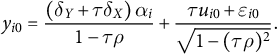$$\begin{align*}y_{i0}=\frac{\left(\delta_{Y}+\tau\delta_{X}\right)\alpha_{i}}{1-\tau\rho}+\frac{\tau u_{i0}+\varepsilon_{i0}}{\sqrt{1-(\tau\rho)^{2}}}. \end{align*}$$

To focus on the essential aspects, the individual units are sampled independently but are distributed heterogeneously as implied by the following assumption.Footnote ⁶

It seems plausible that the simultaneous presence of FE and a feedback effect as described in Equations (1) and (2) would emerge frequently. One example of this is the analysis of electoral outcomes: Much research is concerned with the question of how the regional variation of a factor $x_{it}$ affects regional electoral outcomes ( $y_{it}$ ), where the DGP may be subject to both feedback effects and unobserved heterogeneity. A feedback effect occurs when $x_{it}$ —say, for example, regional unemployment or demographic composition—depends on past electoral outcomes ( $y_{i,t-1}$ ) and thus on the existing political majorities in the time period between $t-1$ and t. Unobserved heterogeneity may be manifested in the form of unobservable time-constant factors, such as cultural or geographical features. In fact, three of the research papers mentioned in the introduction, in which FE and LDV models are estimated and reference is made to the bracketing property, are directly concerned with the analysis of electoral outcomes: Marsh (Reference Marsh2023) analyzes the effects of traumatic events such as arson, mass shootings or natural disasters on voter turnout, Keele et al. (Reference Keele, Cubbison and White2021) analyze the impact of voting restrictions on voter registration, and Tomberg et al. (Reference Keele, Cubbison and White2021) analyze the impact of the presence of refugees on election outcomes.

If FE and a feedback effect are simultaneously present, the estimate of $\tau $ from fitting either an FE model ( $\dddot {y}_{it}=\tau \dddot {x}_{it}+error$ with $\dddot {\cdot }$ indicating within-transformation of the respective variable, for example, $\dddot {y}_{it}=y_{it}-\frac {1}{T}\sum _{t=1}^T y_{it}$ ) or a LDV model ( $y_{it}=intercept+\omega y_{i,t-1}+\tau x_{it}+error$ ) will be biased. As derived for our setup in Section A.2 of the Supplementary Material, these biases (denoted by $B^{FE}_{\tau }$ and $B^{LDV}_{\tau }$ ) are analytically tractable and can be simplified as summarized in the following.

Proposition 1 Under Assumptions 1 and 2, as $N\to \infty $ , we have

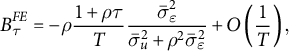(3) $$ \begin{align} B^{FE}_{\tau}=-\rho\frac{1+\rho\tau}{T}\frac{\bar{\sigma}^2_\varepsilon}{\bar{\sigma}^2_{u}+\rho^2\bar{\sigma}^2_{\varepsilon }}+O\left(\frac{1}{T}\right), \end{align} $$

and

(4) $$ \begin{align} B^{LDV}_{\tau}=\frac{\delta_X\delta_Y\sigma^2_\alpha(\tau^2\bar{\sigma}^2_u+\bar{\sigma}^2_\varepsilon)}{(\bar{\sigma}^2_u+\delta^2_X\sigma^2_\alpha)(\rho^2\bar{\sigma}^2_u+\bar{\sigma}^2_\varepsilon)+\bar{\sigma}^2_u\sigma^2_\alpha\frac{1+\tau\rho}{1-\tau\rho}(\delta_Y+\tau\delta_X)^2}, \end{align} $$

where $O(\cdot )$ denotes the order of magnitude.Footnote ⁷

Let us take the approximation in Equation (3) at face value. For the bracketing property to hold in this case, it is necessary that $sign(B^{FE}_{\tau }) \neq sign(B^{LDV}_{\tau })$ , that is, the signs of $B^{FE}_{\tau }$ and $B^{LDV}_{\tau }$ must always be in opposite directions for all combinations of different values for $\rho , \tau , \bar {\sigma }^2_\varepsilon , \bar {\sigma }^2_u, \sigma _\alpha , \delta _X$ , and $\delta _Y$ in the DGP. Yet, it is clearly visible that the sign of $B^{FE}_{\tau }$ depends on the sign of $\rho $ , while the sign of $B^{LDV}_{\tau }$ depends on the sign of $\delta _X \times \delta _Y$ . Thus, as illustrated in Table 1, the bracketing property only holds if $\rho $ and $\delta _X \times \delta _Y$ have the same signs. As discussed in Section 7, whether this is the case is likely to be difficult to determine in most practical applications.

Table 1 Illustration of the conditions under which the bracketing property holds, that is, $sign(B^{FE}_{\tau }) \neq sign(B^{LDV}_{\tau }).$

If the signs are the opposite, then the bracketing property does not hold, that is, both the FE and the LDV estimates of $\tau $ lie above or below the true value of $\tau $ . This means that the bracketing property fails given a DGP in which y and x are positively selected on the FE $\alpha _i$ while the feedback effect is negative, that is, the treatment is negatively selected on past realizations of the outcome. Moreover, the bracketing property fails given a DGP in which y is positively selected on the FE, while x is negatively selected on the FE and the feedback effect is positive.

The following section confirms the predictions of Table 1 using Monte Carlo simulations.

4 Simulation Evidence

To illustrate these theoretical results, we conduct a Monte Carlo simulation that demonstrates the performance of the FE and LDV estimators given a DGP containing FE as well as feedback effects. As a comparison, we also investigate the performance of an OLS estimator ( $y_{it}=intercept+\tau x_{it}+error$ ) as well as an FE-LDV estimator that includes both FE and an LDV ( $\ddot {y}_{it}=\omega \ddot {y}_{i,t-1}+\tau \ddot {x}_{it}+error$ )Footnote ⁸ , which is known to suffer from Nickell bias.

As a starting point, we parameterize the DGP described by Equations (1) and (2) as follows: The FE $\alpha _i$ is generated as a random variable drawn from a normal distribution with mean $~=0$ and standard deviation $~=1$ [ $N(0,1)$ ] once for each individual and remains constant over time. Then, $\varepsilon $ , the error term affecting y, and u, the error term affecting x, are both i.i.d. and drawn from a $N(0,1)$ distribution. The starting values for the dynamic process are i.i.d. draws from a $N(0,1)$ distribution. Following Chudik and Pesaran (Reference Chudik and Hashem Pesaran2019), we discard the first 50 simulated periods to avoid an influence of the starting values on the simulation results, such that $y_{0i}$ may be seen as being drawn from the stationary distribution.

Our parameterization of the DGP is intentionally very simplified to make the simulation results as comprehensible as possible. Therefore, the simulation results can only be interpreted in terms of the presence and direction of the bias. The reader should not over-interpret the magnitude of the bias in the simulated estimators, as the magnitude depends strongly on the underlying parameterization, for which there is an infinite number of different possible combinations.

4.1 Evidence for Bracketing

To illustrate the bracketing relationship, we simulate scenarios in which either the assumptions underlying the LDV model or those underlying the FE model are fulfilled, with the results of these simulations being reported in Tables 2 and 3. Scenarios A to D in Table 2 are based on DGPs that contain a feedback effect of lagged outcomes $y_{i,t-1}$ on contemporaneous $x_{it}$ , but there are no FE. In this case, the LDV and OLS estimators are unbiased, as they only require contemporaneous exogeneity of x, which holds here. In contrast, the estimate of the FE model is biased owing to the violation of strict exogeneity due to the feedback effect. The estimate of the FE-LDV model is also biased due to two channels: the standard Nickell bias of order $1/T$ that applies to the estimator of the autoregressive (AR) coefficient, and, as we show below, a secondary Nickell bias of order $1/T^2$ that applies to the coefficients of the remaining explanatory variables.

Table 2 Monte Carlo simulation results if the LDV model is correct, that is, $\rho \neq 0$ and there are no fixed effects: $\delta _X = 0 = \delta _Y$ .

Note: Results based on Monte Carlo Simulations with 500 repetitions, 300 individuals and 6 time periods. The data generating process is defined by Equations (1) and (2). The variables $\alpha _i, \varepsilon _{it}, u_{it}$ and $y_{i1}$ are all i.i.d. draws from a normal distribution with mean $~=0$ and standard deviation $~=1$ . To mitigate the potential influence of the starting value $y_{i1}$ on the simulation results, we simulate 50 additional time periods and discard the first simulated 50 periods prior to estimating  $\tau $ .

Table 3 Monte Carlo simulation results if the fixed effects model is correct, that is, $\delta _X \neq 0 \neq \delta _Y$ and there is no feedback effect: $\rho = 0$ .

Note: See notes to Table 2.

Next, the data underlying Scenarios E to H is generated by a DGP that includes an FE that simultaneously influences y and x. As expected, the OLS estimator is biased in all cases, as ignoring FE leads to omitted variable bias (Table 3). The LDV model suffers from the same bias. Conversely, the FE model eliminates this bias and yields correct estimates of the treatment effect. The FE-LDV model again suffers from Nickell bias.

To exemplify the validity of the bracketing relationship, we employ the definition given by Angrist and Pischke (Reference Angrist and Pischke2009, 246) and focus on the results of Scenario B presented in Table 2 and the results on Scenario F reported in Table 3. According to Angrist and Pischke (Reference Angrist and Pischke2009), for positive treatment effects, $\tau> 0$ , the bracketing property reads as follows: If the LDV-model “is correct, but you mistakenly use FE, estimates of a positive treatment effect will tend to be too big. On the other hand, if [the fixed effects model] is correct and you mistakenly estimate an equation with lagged outcomes, [...] estimates of a positive treatment effect will tend to be too small.” This definition is summarized in the following Table 4.

Table 4 Illustration of the direction of biases that lead to the bracketing property as described by Angrist and Pischke (Reference Angrist and Pischke2009).

Given the treatment effect estimate $\hat \tau _{LDV}=$ 0.80 resulting from mistakenly estimating an LDV model while the FE model is correct (Scenario F in Table 3), and the alternative estimate $\hat \tau _{FE}=$ 1.03 resulting from mistakenly estimating an FE model while the LDV model is correct (Scenario B in Table 2), the bracketing property holds, as claimed by Angrist and Pischke (Reference Angrist and Pischke2009):

$$\begin{align*}\hat \tau_{LDV}= 0.80 < \tau = 1 < \hat \tau_{FE}= 1.03. \end{align*}$$

We focused in this exemplary illustration of the bracketing property on scenarios in which the feedback effect is negative (Scenario B) or treatment is negatively selected on the FE (Scenario F), because Angrist and Pischke (Reference Angrist and Pischke2009) use an example in which the treatment is a government-sponsored training program that targets individuals with poor labor market outcomes in the past. If contemporaneous labor market outcomes are the outcome variable of interest, such a selection process is represented by a negative feedback effect ( $\rho <0$ , Scenario B) or a negative selection of treatment on unobservable “ability” ( $\delta _X<0$ , Scenario F), which may subsume factors such as intelligence that are largely constant across reasonable observation windows.

A more general definition of the bracketing property is provided in Guryan (Reference Guryan2001, p. 55), who explicitly specifies how the bracketing property depends on the signs of $\rho $ and $\delta _X$ : “if treatment is positively (negatively) selected on lagged outcomes, [that is, if $\rho> 0$ ( $\rho < 0$ ),] the difference in-differences [or the FE] estimator produces negatively (positively) biased estimates of the treatment effect.” Moreover, “if treatment is positively (negatively) selected on fixed characteristics, [that is, if $\delta _X> 0$ ( $\delta _X < 0$ ),] the estimator that controls for lagged outcomes produces positively (negatively) biased estimates of the treatment effect.”

Based on this summary in Guryan (Reference Guryan2001), the bracketing property is entirely confirmed by our simulation results, as presented in the following Table 5.

Table 5 Illustration of how the bracketing property manifests itself in our simulation results.

4.2 Evidence against Bracketing if the FE-LDV Model Holds True

Having established that our DGP is in line with the bracketing property of LDV and FE models, we now allow for both an FE that influences y and x and a feedback of lagged outcomes $y_{i,t-1}$ on contemporaneous $x_{it}$ . As predicted by the analytical results in Section 3, the figures in Table 6 illustrate that all estimates are biased and that the bracketing property no longer holds generally, although in Scenarios A, D, E, and H, the true effect lies within the FE and the LDV estimates.

Table 6 Monte Carlo simulation results when there is a feedback effect of $y_{i,t-1}$ on $x_{it}$ and a fixed effect simultaneously influences $y_{it}$ and $x_{it}$ .

Note: See notes to Table 2.

However, in Scenarios B, C, F, and G, the true effect is not bracketed by the estimates of the FE and the LDV models, as these estimates are both either above or below the true value of $\tau $ . When examining the parameters entered into the DGP for these models, it becomes apparent that these are precisely the situations for which we predict the bracketing property not to hold based on the analytical expressions of the biases (see Table 1).

5 Deriving a Lower Bound from the FE-LDV Model

Our results so far show that the bracketing property afforded by the FE and the LDV models does not generally hold in the presence of unobserved heterogeneity and feedback effects. Hence, when there is a concern that the DGP is characterized by both these features simultaneously, relying on bracketing to identify the upper and lower bounds of the estimated treatment effect is ill-advised. Nevertheless, the results from the simulations suggest that it is at least possible to identify a lower bound estimate: Regardless of the DGP, the FE-LDV model always yields an estimate that is in absolute terms lower than the true coefficient, thus providing a lower bound of the true causal effect of x on y.

To confirm this pattern, we explored several DGPs with different parametrizations and found no instances in which the FE-LDV estimate is either larger than the true causal effect in absolute terms or in which it has a different sign than the true causal effect. These robustness tests are documented in Section B.1 of the Supplementary Material and include variations in the intensity of the feedback effects (Table A3 in the Supplementary Material), the introduction of a dependence between the magnitude of the FE ( $\alpha _i$ ) and the feedback effect (Table A4 in the Supplementary Material), and variations in the noise levels, that is, the standard deviations of $\epsilon _{it}, \alpha _t, u_{it}$ (Table A5 in the Supplementary Material). Apart from noting that none of these changes to the DGP alter the key findings from our main simulation specification, the potential to draw generalizable conclusions from our robustness tests is limited, as the behavior of the estimates is highly dependent on the particular parametrization. Nonetheless, in the cases where a direct comparison is possible, the response of our simulation results to changes in DGP proves to be consistent with the theoretical predictions from Equations (3) and (4) as well as Equation (6) derived below. For example, stronger feedback effects seem to be associated with a stronger downward bias in the FE-LDV estimate, but only when $sign(\tau )=sign(\rho )$ , otherwise it is the other way around (Table A3 in the Supplementary Material), and we find that a relative increase in the standard deviation of $u_{it}$ tends to reduce the bias of all estimators (Table A5 in the Supplementary Material).

In the following, we analytically derive the bias of the FE-LDV estimator of $\tau $ (denoted by $B_{T}^{FE-LDV}$ ) for any T. Starting with $T=3$ , the bias is given by the following expression.Footnote ⁹

Proposition 2 Under the Assumptions of Proposition 1 it holds as $N\to \infty $ that

$$\begin{align*}B_{3}^{FE-LDV}=-\frac{\frac{1}{4}\tau\bar{\sigma}_{u}^{2}\bar{\sigma}_{\varepsilon}^{2}}{\bar{\sigma}_{u}^{2}\frac{\tau^{2}\bar{\sigma}_{u}^{2}+\bar{\sigma}_{\varepsilon}^{2}}{1-\tau^{2}\rho^{2}}-\frac{1}{4}\tau^{2}\bar{\sigma}_{u}^{4}}=-\tau\frac{1}{\tau^{2}\frac{\bar{\sigma}_{u}^{2}}{\bar{\sigma}_{\varepsilon}^{2}}\left(\frac{4}{1-\tau^{2}\rho^{2}}-1\right)+\frac{4}{1-\tau^{2}\rho^{2}}}. \end{align*}$$

This expression highlights that the bias of the FE-LDV estimator is negative for positive $\tau $ and positive for negative $\tau $ , respectively. In turn, this hinges on the condition that $|B^{FE\text {-}LDV}_{\tau }|\leq |\tau |$ . Should this not be met, the FE-LDV estimator would provide an estimate of $\tau $ that has the wrong sign, which would critically limit the applicability of the FE-LDV estimator to provide a lower bound estimate. The condition $|B^{FE\text {-}LDV}_{\tau }|\leq |\tau |$ translates into:

(5) $$ \begin{align} \tau^{2}\frac{\bar{\sigma}_{u}^{2}}{\bar{\sigma}_{\varepsilon}^{2}}\left(\frac{4}{1-\tau^{2}\rho^{2}}-1\right)+\frac{4}{1-\tau^{2}\rho^{2}}>1, \end{align} $$

which holds true generally, since $\tau ^{2}\frac {\bar {\sigma }_{u}^{2}}{\bar {\sigma }_{\varepsilon }^{2}}>0$ and $\frac {4}{1-\tau ^{2}\rho ^{2}}>4 ~ \forall \left |\tau \rho \right | < 1$ .

While these considerations may be repeated for any T, the corresponding expressions become less tractable as T increases, and we consider an approximation following the lines of Nickell (Reference Nickell1981). The result takes the following form.

Proposition 3 Under the Assumptions of Proposition 1 it holds as $N\to \infty $ that

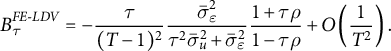(6) $$ \begin{align} B^{FE\text{-}LDV}_{\tau}=-\frac{\tau}{(T-1)^2}\frac{\bar{\sigma}^2_\varepsilon}{\tau^2\bar{\sigma}^2_u+\bar{\sigma}^2_\varepsilon}\frac{1+\tau\rho}{1-\tau\rho}+O\left(\frac{1}{T^2}\right). \end{align} $$

Interestingly, this bias in the estimator of the effect $\tau $ vanishes at rate $1/(T-1)^2$ , which is an order of magnitude faster than the Nickell bias in the FE-LDV estimator of the AR coefficient, which is itself inversely proportional to T. This somewhat surprising finding is, to the best of our knowledge, new, and it is of immediate relevance to practitioners interested in identifying the causal effect of a treatment. The standard expression for Nickell bias, which is of order $1/T$ , applies only to the AR coefficient, and does not in general carry over to other explanatory variables, a point often neglected in the applied literature.Footnote ¹⁰ Equation (6) provides an approximate expression for a secondary Nickell bias that applies to the remaining explanatory variables. We provide a discussion of its relation to Nickell’s original result in Section A.2.2 of the Supplementary Material.

Notwithstanding its speed of convergence, the bias of the FE-LDV estimator is negative for positive $\tau $ and positive for negative $\tau $ , respectively, and thus suggests that the FE-LDV estimator may indeed provide a lower bound estimate for $T>3$ as well. The condition $|B^{FE\text {-}LDV}_{\tau }|\leq |\tau |$ simplifies to:

(7) $$ \begin{align} \tau\rho \leq 1-\frac{2}{1+(T-1)^2\frac{\tau^2\bar{\sigma}^2_u+\bar{\sigma}^2_\varepsilon}{\bar{\sigma}^2_\varepsilon}}, \end{align} $$

which almost certainly holds as long as T is large and the time series of y is stationary, that is, $-1<\tau \rho <1$ .

What about if T is small? We have seen that the condition $|B^{FE\text {-}LDV}_{\tau }|\leq |\tau |$ holds for $T=3$ irrespective of the actual persistence. Moreover, we simulate scenarios with low T and $\tau \rho $ close to unity in Table A1 in the Supplementary Material. In these simulations the bias of the FE-LDV model does not even get close to the size of $\tau $ , supporting the analytical results.

To illustrate the behavior of the estimators at different T and in the presence of FE and feedback effects, we present our simulation results using the parametrization from Table 6 over different values of T in Section B.5 of the Supplementary Material (Figure A2). It can be seen that the biases of the OLS and LDV models are not affected by increasing T, so these estimators do not approach the true effect as T increases. In contrast, both the FE and FE-LDV estimators converge toward the true effect. While they are approximately equidistant from the true value of $\tau $ at $T=3$ , the bias of the FE-LDV estimator vanishes quickly and is relatively close to the true effect from $T=20$ in our simulated case, while this convergence takes longer for the FE model. In line with our theoretical results, the FE-LDV model converges to the correct value from below in all simulated cases, while the FE model sometimes converges from below (Scenarios A and B) and sometimes from above (Scenarios C and D).

Concluding, when suspecting the simultaneous presence of FE and a violation of strict exogeneity due to a feedback effect, referencing the FE-LDV model avails the practitioner with a conservative estimate of the treatment effect, including when T is small—although in this case a substantial underestimation of the treatment effect is to be expected. Indeed, we would caution against trying to discern an upper bound, even in cases where one seems apparent. In Scenario A from Table 6, for example, where the FE-LDV estimate is above the FE and below the LDV estimates, the LDV model cannot be interpreted unambiguously as an upper bound. This is because all estimates could be downward biased while the FE-LDV estimate lies coincidentally between the FE and LDV estimates, a particular case that is presented in Scenario A in Table A2 of the Supplementary Material. Similarly, if the FE-LDV estimate is below both the FE and the LDV estimate, as in Scenario C from Table 6, it again cannot be guaranteed that the LDV estimate is an upper bound estimate, as all estimates may be downward biased, a case presented in Scenario B from Table A2 in the Supplementary Material.

6 The Implications of State Dependence and Nonstationarity

One natural extension of our DGP is to include state dependence in $y_{it}$ , that is, to allow $y_{it}$ to be directly influenced by $y_{i,t-1}$ . This changes Equation (1) to:

(8) $$ \begin{align} y_{it}&=\delta_Y \alpha_i+\pi y_{i,t-1}+ \tau x_{it}+\varepsilon_{it}. \end{align} $$

This DGP requires the stationarity condition $|\pi +\tau \rho |<1$ , reflecting that $y_{it}$ now depends on $y_{i,t-1}$ both directly (via $\pi y_{i,t-1}$ in Equation (8)) and indirectly (via the feedback to $\tau x_{it}$ ).

The simulations based on this DGP (setting $\pi $ to $0.2$ ), are presented in Tables A3, A4, and A5 in the Supplementary Material. Note that the OLS and FE models are still estimated as static models, that is, not including $y_{i,t-1}$ among the regressors. There are several important takeaways from this extension of the DGP: First, in the case where there are no FE but a feedback effect of $y_{i,t-1}$ on $x_{it}$ , the inclusion of a direct effect of $y_{i,t-1}$ on $y_{it}$ in the DGP leads to bias in the OLS estimates (Table A3 in the Supplementary Material), which were unbiased before (Table 2). This is intuitive, as the omission of $y_{i,t-1}$ , which is now correlated with $y_{it}$ as well as $x_{it}$ , leads to omitted variable bias due to the correlation between the error term and $x_{it}$ .

Second, somewhat surprisingly, given state dependence, the static FE estimator is also biased if there are FE but no feedback effect of $y_{i,t-1}$ on $x_{it}$ (compare Table A4 in the Supplementary Material with Table 3). The intuition for this bias was recently laid out by Klosin (Reference Klosin2024): Omitting the LDV in the estimating equation leads to $\varepsilon _{i,t+1}$ being a function of $y_{it}$ and thus of $x_{it}$ . This violates the assumption of strict exogeneity required by the FE model. The upshot, demonstrated in Scenarios F and G in Table A4 in the Supplementary Material, shows that it is not even necessary for both FE and a feedback effect to be present for the bracketing property to be violated. Even with a completely random $x_{it}$ , the bracketing property of FE and LDV can fail if the DGP contains state dependence.

A further result that calls for caution, especially when interpreting the FE model, can be found in Figure A3. There we show the behavior of the different estimators in the face of feedback effects, FE, and state dependence over different observation periods T. Scenarios A - in which FE and LDV would actually bracket the true effect in the absence of state dependence - and B show that the FE estimator changes its sign with increasing T. This means that while the FE and LDV models bracket the true effect in Scenario A at low T, they fail to do so at higher T. Analogously, in Scenario B the two estimators do not bracket the true effect at low T, while they do so at higher T. This supports our conclusion that the presence of state dependence makes a bracketing approach profoundly unreliable.

As in the case without state dependence, the estimates of the FE-LDV model are consistently below the true effect in absolute values. We corroborate these with theoretical results established in the Technical Appendix of the Supplementary Material and summarized below.

Proposition 4 Let $y_{it}$ be generated as in (8) with $x_{it}$ given by (2), where

$$\begin{align*}y_{i0}=\frac{\left(\delta_{Y}+\tau\delta_{X}\right)\alpha_{i}}{1-(\pi+\tau\rho)}+\frac{\tau u_{i0}+\varepsilon_{i0}}{\sqrt{1-(\pi+\tau\rho)^{2}}} \end{align*}$$

s.t. $|\pi +\tau \rho |<1$ and $u_{it}, \varepsilon _{it}$ and $\alpha _i$ obey Assumption 2. Then, it holds as $N\to \infty $ that

$$\begin{align*}B_{T}^{FE}=\rho\frac{\bar{\sigma}_{\varepsilon}^{2}\left(-\frac{1}{T}\frac{1}{1-(\pi+\tau\rho)}\right)}{\left(\rho^{2}\frac{\tau^{2}\bar{\sigma}_{u}^{2}+\bar{\sigma}_{\varepsilon}^{2}}{1-(\pi+\tau\rho)^{2}}+\bar{\sigma}_{u}^{2}\right)}+\pi\left(\rho\frac{\frac{\tau^{2}\bar{\sigma}_{u}^{2}+\bar{\sigma}_{\varepsilon}^{2}}{1-(\pi+\tau\rho)^{2}}\left(1-\frac{1}{T}\frac{1+(\pi+\tau\rho)}{1-(\pi+\tau\rho)}\right)}{\left(\rho^{2}\frac{\tau^{2}\bar{\sigma}_{u}^{2}+\bar{\sigma}_{\varepsilon}^{2}}{1-(\pi+\tau\rho)^{2}}+\bar{\sigma}_{u}^{2}\right)}+\tau\frac{\bar{\sigma}_{u}^{2}\left(-\frac{1}{T}\frac{1}{1-(\pi+\tau\rho)}\right)}{\left(\rho^{2}\frac{\tau^{2}\bar{\sigma}_{u}^{2}+\bar{\sigma}_{\varepsilon}^{2}}{1-(\pi+\tau\rho)^{2}}+\bar{\sigma}_{u}^{2}\right)}\right)+O\left(\frac{1}{T}\right), \end{align*}$$

$$\begin{align*}B_{T}^{LDV}=\frac{\delta_{X}\delta_{Y}\sigma_{\alpha}^{2}\left(\tau^{2}\bar{\sigma}_{u}^{2}+\bar{\sigma}_{\varepsilon}^{2}\right)}{\left(\bar{\sigma}_{u}^{2}+\delta_{X}^{2}\sigma_{\alpha}^{2}\right)\left(\tau^{2}\bar{\sigma}_{u}^{2}+\bar{\sigma}_{\varepsilon}^{2}\right)+\bar{\sigma}_{u}^{2}\sigma_{\alpha}^{2}\frac{1+(\pi+\tau\rho)}{1-(\pi+\tau\rho)}\left(\delta_{Y}+\tau\delta_{X}\right)^{2}}, \end{align*}$$

and

$$\begin{align*}B_{T}^{FE-LDV}=-\frac{\tau}{\left(T-1\right)^{2}}\frac{\bar{\sigma}_{\varepsilon}^{2}}{\left(\tau^{2}\bar{\sigma}_{u}^{2}+\bar{\sigma}_{\varepsilon}^{2}\right)}\frac{1+(\pi+\tau\rho)}{1-(\pi+\tau\rho)}+O\left(\frac{1}{T^{2}}\right). \end{align*}$$

Compared to the baseline case without explicit state dependence, the expressions for $B_{T}^{LDV}$ and $B_{T}^{FE-LDV}$ do not change significantly, in fact the only difference is that now $\pi +\tau \rho $ is the relevant persistence parameter. Only the expression of $B_{T}^{FE}$ changes compared to Proposition 1, given that the FE model is misspecified when there is direct state dependence and the bias now has two sources, namely the omission of $y_{i,t-1}$ as well as the lack of strict exogeneity of $x_{it}$ . Notwithstanding this change, the conclusions about the validity of the bounding behavior do not change.

A further relevant extension consists in relaxing the stationarity assumption. In particular, we consider nonstationarity in form of a unit root, $\pi +\tau \rho = 1$ . Detailed derivations pertaining to this case are provided in the Technical Appendix of the Supplementary Material, and the following proposition shows that the bias of the FE-LDV estimator behaves qualitatively the same even under nonstationarity.

Proposition 5 Let $y_{it}$ be generated as in (8) with $x_{it}$ given by (2), $\pi +\tau \rho = 1$ , and $u_{it}, \varepsilon _{it}$ and $\alpha _i$ obey Assumption 2. Then, it holds as $N\to \infty $ that

$$\begin{align*}B_{T}^{FE-LDV}=-\tau\frac{\bar{\sigma}_{\varepsilon}^{2}}{\frac{1}{3}\left(\left(\delta_{Y}+\tau\delta_{X}\right)^{2}\sigma_{\alpha}^{2}(T-1)T+\left(\tau^{2}\bar{\sigma}_{u}^{2}+\bar{\sigma}_{\varepsilon}^{2}\right)(4T-3)\right)-\tau^{2}\bar{\sigma}_{u}^{2}}. \end{align*}$$

Like above, the direction of the bias is opposite to that of the effect $\tau $ . The exact expression of the bias does differ from the stationary case. One interesting difference is that the unobserved heterogeneity $\alpha _i $ does play a role in the limit. In fact, the rate at which the bias vanishes as $T\to \infty $ depends on whether unobserved heterogeneity is present in the model. If this is not the case (i.e., $\delta _Y=0$ and $\delta _X=0$ ), the rate of convergence is $1/T$ as opposed to the rate of convergence of $1/T^2$ that we found for all other settings. On the other hand, the initial conditions $y_{i0}$ need not be restricted in any way, as they are eliminated by the FE transformation. Nevertheless, it is evident that the bias is smaller in magnitude than the effect for any $T\geq 3$ and the overall conclusion does not change.

Section B.3 of the Supplementary Material contains simulation results for the case of a unit root ( $\rho =1,~\tau =1,~\pi =0$ ) and confirms the theoretical results: The FE-LDV model continues to provide an estimate that is consistently lower in absolute terms than the true effect. In addition, when comparing, for example, Scenario A in Table A9 in the Supplementary Material to Scenario A in Table A10 in the Supplementary Material, that is, once without and once with an effect of unobserved heterogeneity on X and Y at constant T, the simulation results confirm that the bias of the FE-LDV model is actually larger if there is no effect of unobserved heterogeneity.

7 Practical Implications

Returning to the initial question “so what’s an applied guy to do?” (Angrist and Pischke Reference Angrist and Pischke2009, 245), the key implication of our results is that the bracketing property is not a panacea in situations where empirical researchers are concerned with confounding by unobserved time-constant heterogeneity as well as violations of the assumption of strict exogeneity, for example because of feedback effects or state dependence. This is because the bracketing property is only reliable if either strict exogeneity holds or there is no confounding by unobserved time-constant heterogeneity. Given the likely uncertainty surrounding this issue, it may be possible to avail diagnostics tests that allow the researcher to rule out one source of bias or the other. For example, unobserved time-constant heterogeneity can be explored using tests in the spirit of Hausman’s (Reference Hausman1978) specification test (Frondel and Vance Reference Frondel and Vance2010), while statistical tests for the strict exogeneity assumption are proposed by Wooldridge (Reference Wooldridge2010, p. 285). The outcome of such an exercise may clearly point to the preferability of the FE or LDV model, as would be the case if either the strict exogeneity assumption is violated or an FE model is required. Bracketing in this case is unnecessary.

Another case in which there is clarity about the path forward is the two-period setting with a binary treatment covered by Ding and Li (Reference Ding and Li2019). The authors propose a test in which the cumulative distribution function (CDF) of the pre-treatment outcome variable for the treatment and the control group are plotted against each other (see Keele et al. (Reference Keele, Cubbison and White2021) for an application). If one CDF is monotonically above/below the other (stochastic monotonicity), Ding and Li’s (Reference Ding and Li2019) results imply that the bracketing property is likely to hold.

However, if one moves away from the two-period difference-in-differences setting with binary treatment, this approach reaches its limits. As our analysis has shown, with multiple periods, bracketing only works if the selection of the independent variable of interest x depends in the same direction, that is, positively or negatively, on lagged outcomes and the relevant omitted time constant variables ( $sign(\rho ) = sign(\delta _X \times \delta _Y)$ , see Table 1), and if there is no state dependence. One example in which these conditions might be met is the study of Beckmann and Kräkel (Reference Beckmann and Kräkel2022), who, among other identification strategies, estimate FE and LDV models to bracket the effects of work autonomy (x) on work engagement (y). In this case, we might tell a story about an unobservable fixed factor such as ability that makes the sign of $\delta _X \times \delta _Y$ positive, coupled with the expectation that past engagement positively affects today’s autonomy, making $\rho $ positive as well. Under this circumstance, the potential selection of x on FE should go in the same direction as the potential selection of x on past outcomes, supporting bracketing.

Whether such a story is convincing is, of course, open to interpretation. In our view, an analyst will typically be hard-pressed to make an airtight case for bracketing.Footnote ¹¹ We therefore recommend that authors transparently discuss their theoretical considerations on the possible selection process, taking into account our insights from Section 3, and indicate in which of the cases listed in Table 1 they see their setting. If these theoretical considerations lead to an ambiguous result, as we believe will often be the case, authors should not rely on the validity of a bracketing approach. Instead, authors should pay particular attention to the FE-LDV model, which provides a conservative reference point, yielding a lower bound of the true effect, even if the nature of the selection process is unclear. Moreover, we show that the bias of the FE-LDV estimator of the explanatory variables decreases at rate $1/T^2$ (see Proposition 3), so that the results of the FE-LDV model converge relatively fast toward the true effect as T increases.

An empirical example in which the presence of FE, state dependence, and feedback effects would hypothetically render the result of a bracketing approach misleading can be found in Acemoglu et al. (Reference Acemoglu, Naidu, Restrepo and Robinson2019). The authors estimate the effect of democratization on economic growth using a panel of 175 countries from 1960 to 2010. The authors implement several specifications but do not reference bracketing. A key observation, demonstrated descriptively in their Figure 1, is that democratization is often preceded by a decline in GDP, which suggests the presence of a feedback effect with $\rho <0$ . Moreover, they argue persuasively that “democracies differ from nondemocracies in unobserved characteristics, such as institutional, historical, and cultural aspects” (p. 49). Together, these considerations lead the authors to estimate dynamic panel data models, including an FE-LDV model, throughout the paper. Using the replication files of Acemoglu et al. (Reference Acemoglu, Naidu, Restrepo and Robinson2019), we estimate the results if the authors had tried to bracket the true effect with FE and LDV models, focusing on the simplest specification in column 1 of their Table 2. The estimate of the effect of democratization on log GDP per capita would be 0.457 (0.296) in the LDV model and $-$ 10.112 (4.316) in the FE model (standard errors in parentheses).Footnote ¹² In contrast, their reported and replicable result of the FE-LDV model is 0.973 (0.294), while the result of their preferred specification in column 3, which includes four lags of the dependent variable, is 0.787 (0.226), both falling outside the range of the bracket.

Throughout most of this article, we have assumed contemporaneous exogeneity, that is, zero correlation between $x_{it}$ and $\varepsilon _{it}$ for all t and conditional on accounting for FE. If this condition is not met, conventional approaches to causal inference (e.g., instrumental variables), possibly also in combination with a bracketing approach, should be considered. Furthermore, the dynamic structure that we have adopted in our DGPs is relatively simple, but should cover a wide range of applications. Nevertheless, there may be cases in which deeper lags of the dependent or explanatory variables may be part of the DGP (e.g., Acemoglu et al. Reference Acemoglu, Naidu, Restrepo and Robinson2019). A generalization of our results to these cases and a discussion of the implications for the interpretability of the estimated coefficients, for example, with respect to short-run and long-run effects (Beck and Katz Reference Beck and Katz2011; Keele and Kelly Reference Keele and Kelly2006), is beyond the scope of this article.